So, do you want to master data and gain insights on how your business is growing, while loving to code?

You have come to the right place! Let me introduce you to the topic of exploring data, also known as Data Science.

Data is everywhere and controls everything and as such analyzing it is increasingly important. Insights over the data on a business can be critical and provide an edge on today’s highly competitive market.

Mastering data not only will grant you a future in the modern world, but will also make you a valuable asset for companies.

Today you will learn basic essential data science tools and a base on which you can base on to improve your skills.

This will assume you already have Python 3.10+ installed on your local machine, if not, you can visit the official site here. All the code will written down here.

what do you need?

Assuming that you already have Python installed, we will start looking at one of the most popular packages on the community that focus on Data Science and in Engineering, SkLearn. To install it run the following command.

pip install scikit-learn

This package and a dependency of it, numpy, are the core foundations of data science in Python.

While numpy focus more on handling the data, sklearn takes care of processing it and turning into useful insights.

Before you tackle any problem you will need 2 things, a dataset and a goal.

A dataset is basically data that you will need to process down the line. And, to view and store those datasets I will use yet another library called pandas that can be installed like this.

pip install pandas

This tools will help a lot in our little endeavour and you can think about Data Science like a factory, raw materials in, finished products out. Applying it to our problem, data comes in, insights come out.

When I talk about insights, I mean just information about dataset, be it a simple thing or a really complex analytic.

where to obtain your datasets?

In the topic of obtaining a dataset, you have 2 alternatives, either you build your own or go to a website like Kaggle and download a dataset, or you build your own dataset. Let’s see the pros and cons of both options.

Starting with going to a website and downloading a pre-made dataset can have a lot of advantages, like the ease of starting on a new project and a great variety of choices.

Overall, while choosing a dataset that is available can be very advantageous, you lose the personalization aspect.

And that brings us to the other option, that is building you own dataset using resources found in the web or even with your own resources.

This is the option you would choose in a production environment, since the data you will be using is tailored to your needs and use case.

However it can be really expensive specially if you are taking Data Science as a hobby or to learn.

So, today I will be using a famous dataset from the Titanic incident and we will be analyzing the survival rates based on a few factors.

The dataset can be found in kaggle through this link.

loading the dataset

The dataset comes in a form of an xls file. This file is commonly used in Excel, however we will load it using pandas.

To load it and visualize what it contains, first we need to import the libraries, then call pandas.read_excel to load our data. You may need to install another package called xlrd via pip.

A dataframe (the structure returned by pandas) can be thought as a table with a header and data in rows.

To view it’s contents we can print it or call the method .head. This method will return by default 5 rows, but you can pass an argument to specify how many rows do you want.

Putting all together we have the following code.

import pandas as pd

dataset = pd.read_excel('data/titanic.xls')
print(dataset.head())

You can see now the top 5 rows of the dataset that I placed in the data directory.

doing some basic feature engineering

This dataset has a lot of features or dimensions meaning that we need to filter out and pre-process the features that we need and are relevant. As said before, we will be looking at the survival rates based on some features.

Let’s now see which are the best features to be looking at. For that we can use the features that have the most values, since some of the rows does not include all features.

To extract a column from a dataframe we can index it with the name of the column. So with something like this we can extract the passenger class from the dataset.

print(dataset["pclass"])

Another useful command is the method info of the dataframe that tells us detailed information about each columns, such as the non-null values and the type.

Running that command in the dataset will tell us which features are better candidates to be analyzed. Now we will learn how to filter out the features with low correlation with the feature under analysis.

understanding the data

To visualize the correlation between sample points, we will need to install another package. The name of that package is matplotlib and is installed with pip.

Survival rate

To create a 2D graph we need 2 coordinates, X and Y. Let’s first see the correlation between the passsenger sex and our study subject, survival rate.

For this example, X will be the passenger sex and Y the outcome of the passenger. We can then do a linear regression to fit the data and check for the correlation between the 2.

import numpy as np
from sklearn.linear_model import LinearRegression
import pandas as pd
import matplotlib.pyplot as plt

dataset = pd.read_excel('data/titanic.xls')
print(dataset.info())
print(dataset.head())

X = dataset['sex']
X = X.apply(lambda x: 0 if x == "male" else 1)
y = dataset['survived']

X2 = np.arange(len(X))
lr = LinearRegression()
lr.fit(X2.reshape(-1, 1), y)
pred = lr.predict(X2.reshape(-1, 1))
correlation = np.corrcoef(pred, y)[0, 1]

plt.plot(X2, pred, color='blue')

plt.title('Titanic Survival')
plt.show()
print(correlation)

Which give us something like this for the regression.

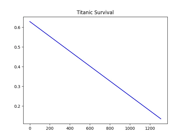
And a value of 0.29 for the correlation, which is not great.

So we conclude that those 2 values are not strongly correlated and as such is not a good candidate.

But let’s now look to another candidate: the age of each passenger.

passenger age

The age has some null values that we will need to discard or process. To process the age we can either set the null values to a fixed value or just discard them or even process it in another ways. I will be discarding them, but feel free to find another way to process it!

This time we have this.

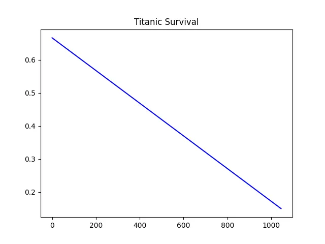
Despite looking the same as before, it has a higher correlation of about 0.30 meaning that it is not enough to draw conclusions in its own. However it can be interesting to analyze in conjuntion with the passenger sex as both have a similar correlation and a similar regression line.

clustering data

Using the same technique as before I identified the fare feature as having a similar result so, I will be using that as well as the other features to cluster.

To cluster data we can use K-Means clustering provided in the sklearn package.

This clustering algorithms works by finding clusters of data, assigning then an identifier to the cluster. Since the result is discrete (either 1 or 0) this works perfectly, with only a single caveat. We need to find which cluster is the 1 and which one is the 0.

To do that we just check the cluster with higher accuracy by just summing all values and dividing by the sample size.

See the example below that grabs those features and performs K-Means Clustering.

import numpy as np
import pandas as pd
from sklearn.cluster import KMeans

dataset = pd.read_excel('data/titanic.xls')
print(dataset.info())
print(dataset.head())
non_null_values = dataset["age"].notnull() & dataset["fare"].notnull() & dataset["sex"].notnull()

Xage = dataset["age"][non_null_values]
Xfare = dataset["fare"][non_null_values]
Xsex = dataset["sex"][non_null_values].apply(lambda x: 1 if x == "male" else 0)

y = dataset["survived"][non_null_values].values.reshape(-1, 1)
X = np.array(list(zip(Xage, Xfare, Xsex)))

cluster = KMeans(n_clusters=2, random_state=0)
cluster.fit(X)

y_pred = cluster.predict(X).reshape(-1, 1)

print("Accuracy: ", np.sum(y == y_pred) / len(y))

Here I am using a random_state of 0 so your results are similar to mine.

As such, with this code you will get around 67% accuracy.

Another important topic is the number of clusters used, meaning the number of classes we have. In this case we used 2 because the situation was binary.

However you can tweak those and much more parameters of the KMeans method, by searching on sklearn website.

conclusion

Pretty wild, isn’t it? Based on how much the people paid, the sex and the age you can have an estimate of whenever the person is going to survive.

You can experiment feeding the predict method your own data and seeing the output.

With that said, today you learned how to perform basic data analysis in python, using sklearn and numpy. Knowing this is going to be something that will boost your career and portfolio.

So, have a great day and thank you for reading my post. See you next time!